LLM Fundamentals - Visualizing Transformer Internals
This is a machine translation of LLM Fundamentals - Visualizing Transformer Internals CN
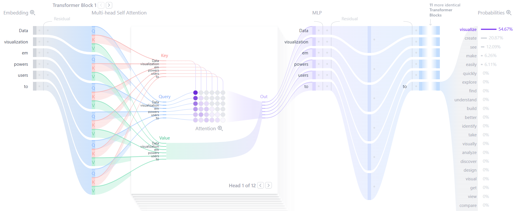
The iteration of large models (Large Language Model, LLM) technology has been like a technological explosion; techniques that were cutting-edge six months ago have now become the basis of the basics. Polo Club created an animated explainer of the Transformer model, which is very helpful for visualizing and understanding how Transformers work. In addition, the DeepSeek-V3 paper was released like a carnival, detailing every aspect from models to infrastructure, and it was open-sourced — even explaining production-grade MoE implementations.
Polo Club Visualization:https://poloclub.github.io/transformer-explainer/
This article was also published on my WeChat Official Account:
- Link: https://mp.weixin.qq.com/s/V_uyS-rOFVia3Mu49QhuHg
- PDF: LLM-Fundamentals-Visualizing-Transformer-Internals-CN.pdf
Citation
DeepSeek-V3 paper:
- [1] DeepSeek-V3 Technical Report: https://arxiv.org/pdf/2412.19437
- [2] DeepSeek infra: https://arxiv.org/html/2408.14158v1
- [3] DeepSeek-R1: https://arxiv.org/pdf/2501.12948
DeepSeek open source:
- [4] Model: https://github.com/deepseek-ai/DeepSeek-V3
- [5] 3FS: https://github.com/deepseek-ai
- [6] More components: https://github.com/orgs/deepseek-ai/repositories?type=all
Overall architecture
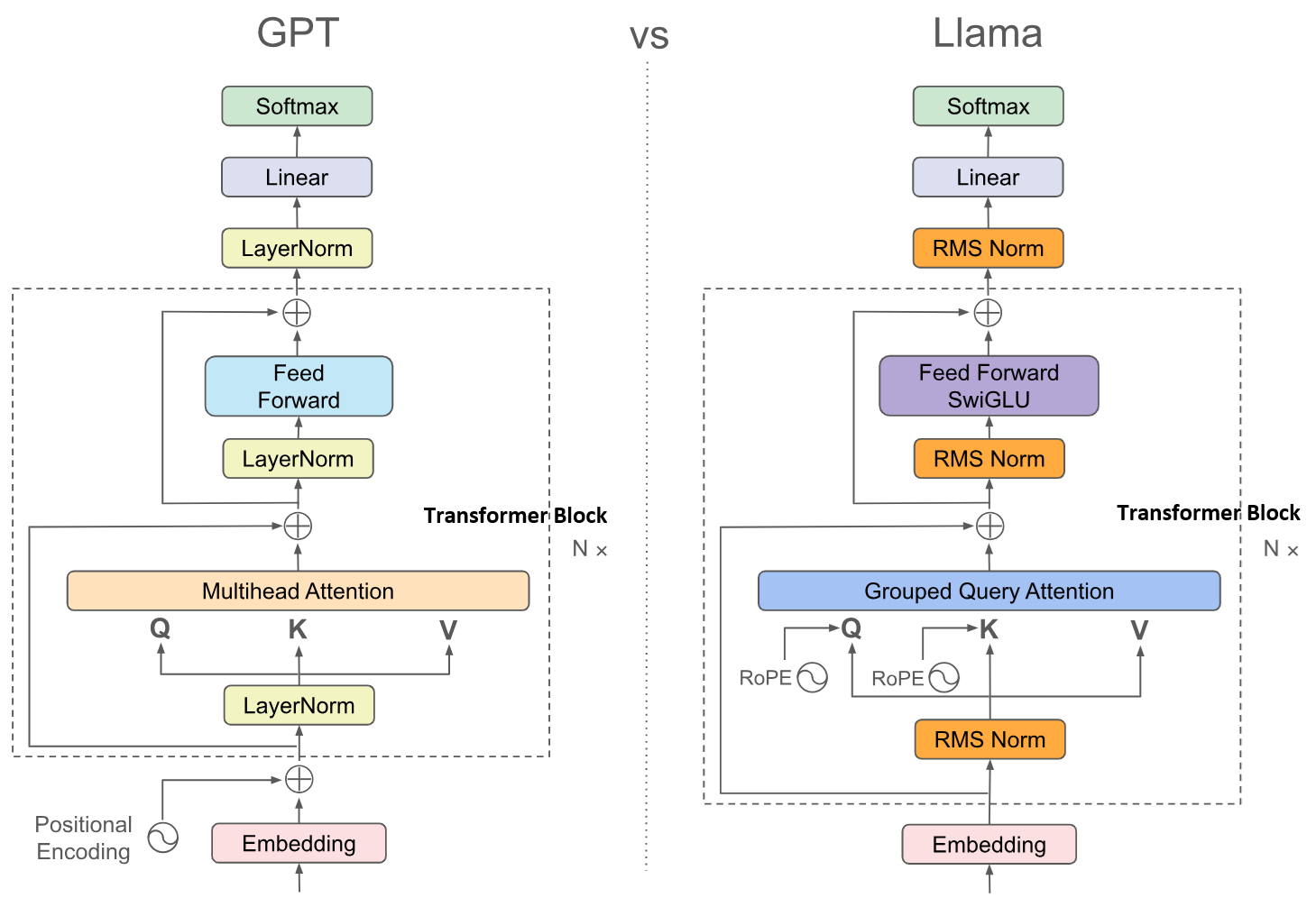
From the above figure, we can see that a Transformer model is essentially a stack of Transformer Blocks (dozens or hundreds). Modern Transformer models are basically decoder-only because they are easier to train and optimize for performance, taking advantage of the scaling laws. Research has long shown that increasing the depth of a neural network is more effective than increasing its width, because a deeper neural network is like a composition of functions with stronger expressive power; each layer can leverage the intermediate results of the previous layer.
Below explains the components in the above diagram:
-
At the Transformer model’s input there is an Embedding layer that performs three tasks: tokenization, token embedding, and positional encoding. Tokenization identifies frequent prefixes and word pieces, so parts like “un”, “ing”, “able” can be recognized as separate tokens. Token Embedding maps token IDs to vectors; its parameters are learned jointly with the Transformer model. Positional encoding, such as sinusoidal encoding, encodes each token’s relative position in the sentence and is fused into the token inputs.
-
In the middle are a stack of Transformer blocks; this architecture has similarities to convolutional neural networks (CNNs) from a few years ago. CNNs are used for image vision processing. Their lower layers learn local and syntactic patterns, while higher layers learn global semantics and reasoning, forming an “abstraction tower.” Attention sits inside each Transformer block and is explained in detail later.
-
Finally, there is the output layer. The vector output by the last Transformer block is multiplied by a large matrix — up-projected (see below) — to a vector the same size as the vocabulary, called the logits. Then the top-K tokens with the largest logits are selected. Finally, a softmax maps the logits to probabilities, and a token is sampled from that distribution as the output. Optionally, before entering softmax the logits can be divided by a temperature value. Higher temperature flattens the probabilities, making the model’s final outputs more random (higher temperature, higher entropy).
Embedding has been used for many years before the Transformer; it converts words into high-dimensional vectors with geometric distances so the model can process them. Positional encoding became widely known together with the Transformer; its mathematics are at once simple and ingenious. The Softmax method in the output layer is commonly used in neural networks. The Transformer Block contains the key to large models, as described below.
Citation
- [7] Why are current LLMs all decoder-only architectures: https://www.zhihu.com/question/588325646
- [8] Why deeper NN is more effective than wider: https://www.reddit.com/r/MachineLearning/comments/h0g83p/d_why_are_deeper_networks_better_than_wider/
- [9] CNN: https://learnopencv.com/understanding-convolutional-neural-networks-cnn/
- [10] Positional Encoding: https://medium.com/thedeephub/positional-encoding-explained-a-deep-dive-into-transformer-pe-65cfe8cfe10b
Transformer Block
What exactly is inside a Transformer Block?
-
First is the Attention module — the source of the Transformer’s magic, which will be explained in detail in later sections. The remaining parts are neural networks and some techniques.
-
Next is the feed-forward network (FFN). “Feed-forward network” is just a grandiose name for the most basic kind of neural network. The network structure is simple and straightforward: input layer -> hidden layer -> output layer, and the hidden layer can have multiple layers. It’s called “feed-forward” because data only flows forward. FFNs are also often called multilayer perceptrons (MLP) or fully connected networks (FCN).
-
RMSNorm (Root Mean Square Normalization), literally normalization using the root mean square. Layers in neural networks are commonly normalized to constrain the range of activations and prevent gradient explosion or vanishing. RMSNorm is gradually replacing LayerNorm as the mainstream for large models. RMSNorm has fewer parameters, is easier to train, and can preserve the direction of vectors (rather than subtracting the mean as LayerNorm does).
-
The next key element is the residual connection, originating from ResNet. Adding a cross-layer connection in deep neural networks can mitigate the harms of depth, prevent information loss and error accumulation, and help gradients propagate through deep layers.
(The image is from the DeepSeek-V3 paper.)

FFN is the foundation of neural networks and has been in use for decades. RMSNorm is also common; the layers of neural networks almost always require normalization. Scaling, normalization, and standardization are standard methods for processing features. Residual connections are simple and effective, and were widely adopted after the introduction of ResNet a few years ago. But Attention is the true original innovation—Attention is all you need.
Citation
- [11] FFN: https://learnopencv.com/understanding-feedforward-neural-networks/
- [12] Normalization: https://2020machinelearning.medium.com/deep-dive-into-deep-learning-layers-rmsnorm-and-batch-normalization-b2423552be9f
- [13] ResNet: https://en.wikipedia.org/wiki/Residual_neural_network
Attention
Attention is the core of the Transformer. The diagram below shows the formula for attention.

The original formula is information-dense. Below, it is expanded into a more ordinary form using code, and then each component is explained line by line.
// Each row of the InputMatrix is an embedding vector of an input token.
// The number of rows is the total number of tokens.
Q = InputMatrix * WeightMatrix_Q
K = InputMatrix * WeightMatrix_K
V = InputMatrix * WeightMatrix_V

// Attention formula
Attention = softmax((InputMatrix * WeightMatrix_Q
      * WeightMatrix_K^T * InputMatrix^T)
    / sqrt(d_k))
  * (InputMatrix * WeightMatrix_V)
The following explains each component in the formula:
-
Input Matrix: A Transformer takes Tokens as input, with each Token represented as a vector (Embedding). A single text input can range from tens to millions of Tokens, and Token vectors can have hundreds to thousands of dimensions. Token vectors are represented as rows, stacked row by row to form the input matrix. (In some papers, Token vectors are represented as columns, and you will see the Attention formula become Q^T * K, with Q = WeightMatrix_Q * InputMatrix; this does not affect the result.)
-
Q = InputMatrix * WeightMatrix_Q: Q stands for Query. Before computing Attention, the input (InputMatrix) is pre-multiplied by a weight matrix WeightMatrix_Q to obtain Q. Processing the input with weights is a common technique; K and V are obtained in the same way. K stands for Key, V stands for Value.
-
QK^T: A square matrix whose dimension equals the total number of Tokens (which can be extremely large); the matrix elements are floating-point numbers (not vectors). Expanded, it takes the form InputMatrix * M * InputMatrix^T. The (i,j) entry of the matrix is the dot product (with weighting) of Token i and Token j. Intuitively, it means the text input (a sequence of Tokens) is looking at itself (multiplying with itself). This is the origin of “self-attention.”
-
Sqrt(d_k):d_k is the dimension of Token vector. Sqrt(d_k) is commonly called “Scaling factor”. Suppose elements in Q and K follows normal distribution N(0,1), then QK^T will increase variance to d_k. To make the variance back to 1, it needs to divide by Scaling factor - sqrt(d_k) 。
-
Softmax: A standard normalization formula commonly used for probabilities, applied row-wise to the input matrix. After softmax, the elements in a row sum to 1, so the row becomes like a probability distribution. QK^T processed with softmax becomes the probability of Token i looking at Token j (self-attention). The softmax formula uses e for the exponential because probabilities are naturally related to exponentials; you can view it in terms of an exponential distribution’s MTBF.
-
V: From the above, softmax(QK^T / sqrt(d_k)) yields the probabilities for self-attention. These probabilities must be multiplied by the input values to obtain outputs of the same dimension. V is the input values (with weights), hence called Value.
In summary, Attention can be seen as applying weights to the token inputs (InputMatrix), where the weights are the self-attention. Note that the weights for Q, K, and V are right-multiplied, so the weighting acts within a single token vector. The self-attention weights are left-multiplied, so the weighting acts across multiple tokens, causing token mixing.
In addition, there are some extra points about Attention:
-
Multi-head: The Attention layer in a Transformer block is Multi-head Attention. That is, multiple attention models run in parallel within the layer; each is called a “head” and has its own parameters, with the total number of heads ranging from a dozen to several dozen. The term “multi-head” may originate from image processing (e.g., CNNs), where handling RGB pixels requires at least three channels — three heads.
-
Masking: If a Transformer supports a 1M-token context, then Attention would theoretically be handling a matrix of dimensions 1M * 1M. In practice, however — see the KV Cache section — Attention is computed one token at a time. If the user input is 1,000 tokens, then when computing the 900th token (Prefill), the remaining 100 tokens need to be zero-padded. That is the first meaning of masking. If the combined user input and output do not fill the full 1M-length context, those unfilled positions also need to be zero-padded. That is the second meaning of masking. Zeros in the softmax computation do not translate to zero probability (e^0 = 1). To get zero probability, the inputs must be changed from zero to negative infinity. That is the third meaning of masking.
References
- [14] Deep understanding Attention mechanism P2: https://medium.com/@funcry/in-depth-understanding-of-attention-mechanism-part-ii-scaled-dot-product-attention-and-its-7743804e610e
A geometric picture of Attention
Attention actually has a very vivid and intuitive geometric picture. With the above foundations, the following gives a deeper explanation of what Attention is doing:
-
Embedding: This is the input to Attention. Embedding converts tokens into vectors to begin Attention computation. These vectors have geometric meaning. If the angle between two vectors is small and their dot product is large, it means the corresponding tokens have similar meanings. Adding vectors can blend meanings to produce a new token, for example king + woman = queen.
-
Q = InputMatrix * WeightMatrix_Q: The token vectors from Embedding do not participate directly in Attention computation; they are first multiplied by the Q weight matrix. Imagine each column of WeightMatrix_Q as another set of embedding vectors — they are rulers. Multiplying them with token vectors measures how close a token is to each ruler. The output Q is the token reconstructed in the coordinate system defined by this set of rulers. WeightMatrix_K works the same way.
-
Positional encoding: Using RoPE as an example, in simplified terms it rotates the token vectors by an angle. The later a token appears in the sentence, the larger the rotation angle. The farther apart two tokens are, the greater the difference in their rotation angles. For two tokens separated by the same distance in the sentence, the difference in rotation angle is always the same regardless of their absolute positions. The smaller the angle difference, the larger the dot product. In this way, positional encoding gives higher Attention scores to neighboring tokens.
-
QK^T: This computes the pairwise dot products of tokens; the dot product is the Attention score (later normalized by sqrt(d) and softmax). Thus, the closer the angles of two token vectors, the closer their meanings and the closer their positions in the sentence, the larger their Attention score will be.
-
V: The Attention computation ultimately multiplies the Attention scores by V; this mixes the token vectors represented by the rows of V. If a token in one row has a higher Attention score toward another token, then that other token receives a higher weight in the mix. In the final Attention output, the original token vector becomes — itself plus the sentence context it “attends” to.
(The diagram omits normalization components such as sqrt(d) and softmax.)
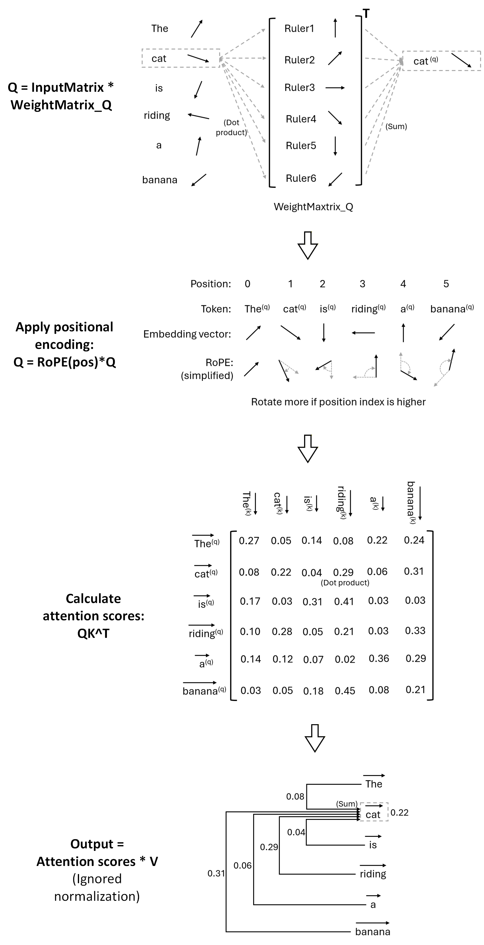
With this geometric interpretation, we can see that Attention scores essentially compute pairwise similarity between token vectors. Without positional encoding, Attention would be permutation-invariant with respect to tokens (i.e., order-independent). Therefore, positional encoding must be introduced.

KV Cache
Another major advantage of Attention is its computational properties. If a Transformer supports a 1M-token context, Attention would theoretically involve multiplying matrices of dimension 1M × 1M. In practice, however, Attention can be implemented incrementally, token by token. Each new token reuses the previous token’s computation — this is the KV Cache.
In the linked figure below, the author created an animated visualization that greatly helps in understanding the KV Cache computation process. You can see:
-
When calculating Token 2, Need to use Value Token 1~2, Key Token 1~2, Query Token 2.
-
When calculating Token 3, Need to use Value Token 1~3, Key Token 1~3, Query Token 3. Value Token 1~2 and Key Token 1~2 can reuse Token 2’s.
-
When calculating Token 4, Need to use Value Token 1~4, Key Token 1~4, Query Token 4. Value Token 1~3 and Key Token 1~3 can reuse Token 3’s.
(KV Cache 动画:https://medium.com/@joaolages/kv-caching-explained-276520203249 )
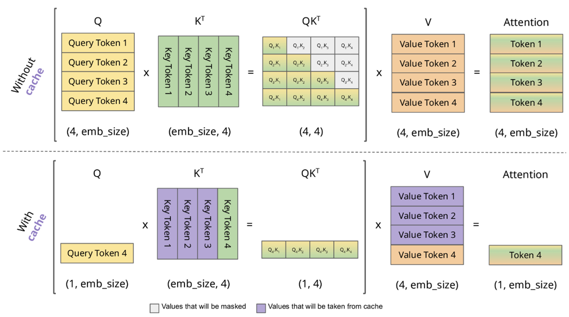
When computing the next token, the full set of Key tokens and Value tokens is always needed; these can be incrementally reused from the previous round’s computations and are therefore suitable to be stored in a cache — hence the KV Cache. The Query, by contrast, only needs the current token and not the full set, so there is no Q Cache.
- You can see that the longer the user input context and the more tokens there are, the larger the required KV Cache becomes proportionally, and the higher the cost. This explains why ChatGPT and similar products tend in their UI design to encourage users to start a new conversation.
Note that the KV cache depends on tokens that were computed previously. If a token in the middle of the context is changed, the later KV cache cannot be reused. This is because a Transformer has many intermediate layers, and each intermediate Transformer block has its own attention and KV cache. Tokens at an intermediate layer come from the attention of the previous layer. Attention’s probability weighting is across tokens, so the values of historical tokens will change the value of the current token.
-
Therefore, the KV cache is often implemented as a prefix cache. The KV cache can only be reused when the prefix (the prior conversation history) is the same.
-
In agent design, the system prompt is always placed at the start of the conversation and its content is always the same. Their KV cache can be reused across conversations and across users.
Because of the KV cache, when using a Transformer for inference (rather than training), it is common to divide the process into a prefill stage and a decode stage. The prefill stage feeds the user’s input text into the Transformer with the goal of generating the KV cache, hence it is called “prefill.” The decode stage occurs after prefill is completed, when the Transformer begins predicting subsequent tokens based on the user’s input and produces the output.
- Prefill and Decode stages have different computational characteristics. In the Prefill stage, the user input is known and systems are designed to maximize parallelism; the bottleneck is usually GPU compute capability. In the Decode stage, tokens must be predicted one by one sequentially, but the KV Cache must be fully stored, so the system bottleneck is often memory (VRAM).
Quote
- [15] Mooncake / Kimi and Prefill / Decode decoupling:https://arxiv.org/pdf/2407.00079
- [16] Cursor about Prompt processing (Prefill stage) and Generation (Decode stage) computation cost : https://cursor.com/blog/llama-inference#a-primer-in-transformer-math
Multi-Head Latent Attention (MLA)
Below is an introduction to the Multi-Head Latent Attention (MLA) from the DeepSeek-V3 paper. The “magic” of MLA is that it reduces KV Cache usage through down-projection compression, thereby improving inference performance. Tests show that this compression has little impact on inference quality.
In the formula in the figure,
-
The vectors in the blue boxes are cached in the KV Cache.
-
h_t denotes the token vector (embedding), which is the input to the attention.
-
The W^D* matrix denotes the down-projection matrix, and the W^U* matrix denotes the up-projection matrix.
-
k, q, v refer respectively to the K, Q, V vectors in attention.
-
In k_t,i, t denotes the t-th token and i denotes the i-th head (multi-head).
-
c* is the latent vector introduced by MLA — a compressed vector hidden in intermediate steps.
-
*R denotes RoPE encoding, used to encode a token’s position in the sentence.
(The image is from the DeepSeek-V3 paper.)
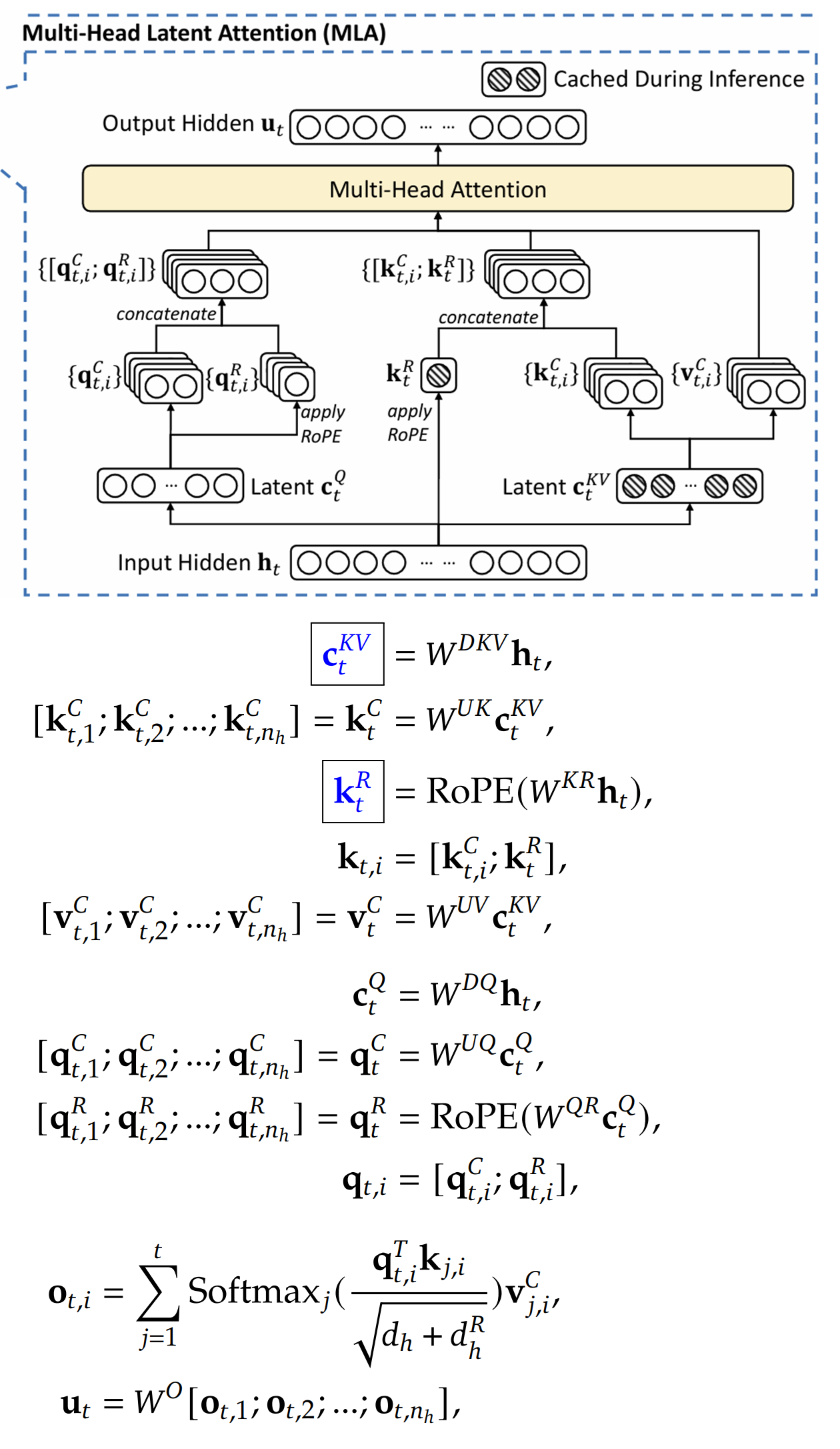
Below I will explain each component of MLA one by one:
-
First look at the right half of the figure. Unlike ordinary Attention which computes K and V directly from h_t, MLA first down-projects h_t to c_t^KV. c_t^KV is cached, rather than caching K and V separately, and there is no need to cache a copy for each head. This reduces KV cache usage. Then c_t^KV is up-projected to recover the K and V needed for the Attention computation, and made multi-headed.
-
Next look at the left half of the figure. The processing of Q is similar: h_t is first down-projected to c_t^Q, and then up-projected to recover the Q vectors needed for the Attention computation. Note that Q does not need to be stored in the KV cache.
-
Observe the parts in the figure marked with R: MLA also adds RoPE positional encodings to the K and Q vectors, producing k_t^R and q_t,i^R. The final vectors input to Attention are formed by concatenating the up-projected vectors with the RoPE-encoded vectors. Note that the RoPE-encoded vectors are only half the length of the former. Also, k_t^R is not multi-headed, which reduces KV cache usage. The trick is similar to MQA, with all heads sharing K.
-
Finally, K, Q, and V are fed into the standard Multi-Head Attention for computation.
As you can see, the key to saving KV Cache lies in down-projection compression. The RoPE positional encoding is routed to a separate path for special handling.
The down-projection compression technique mentioned above appears in multiple aspects of large models and is also called Low-rank Compression, which is quite different from “compression” in storage. For example:
-
Application 1: LoRA is a commonly used fine-tuning technique for large models. The fine-tuned model can be represented as h = W0 * x + ∆W * x = W0 * x + B A * x. The model matrix W0 and the parameter update ∆W are huge in dimension and costly to update. But ∆W can be expressed as the product of two much smaller matrices B * A. The number of columns of B and the number of rows of A can be chosen to be any smaller dimension, making the total number of parameters in B and A far less than that of ∆W. This is why fine-tuning is cheaper than full training.
-
Application 2: MLP Expansion/Compression refers to intermediate layers of a multilayer neural network increasing or decreasing dimensionality. For example, the input vector dimension may be 768, the intermediate layer dimension 3072, and the final output returns to 768. Expressing the neural network in matrix form, this is equivalent to the input vector first being multiplied by an up-projection matrix to increase dimensionality, computation occurring, and then multiplied by a down-projection matrix at the output to reduce it back to the original dimension. The high dimensionality inside the neural network provides capacity for storing knowledge and expressing nonlinearity. This technique is used in the FFN layer of a Transformer Block.
Quote
- [17] Deepseek技术解读(1)-彻底理解 MLA: https://zhuanlan.zhihu.com/p/16730036197
- [18] LoRA paper: https://arxiv.org/abs/2106.09685
Deeper questions about MLA
The above explained the working principle of MLA; next, some deeper questions about MLA can be raised:
Why do RoPE and the down-projection of K and Q need to be computed separately?
-
You can understand it this way: going back to the Attention chapter’s formula, QK^T = InputMatrix * WeightMatrix_Q * WeightMatrix_K^T * InputMatrix^T. Here WeightMatrix_Q * WeightMatrix_K^T can be pre-fused into a matrix M to simplify computation. And M remains unchanged for whichever token it is. But if RoPE is inserted in the middle, since it is position-sensitive, M no longer has a fixed value and the computation cannot be simplified.
-
Using the paper’s explanation: RoPE is incompatible with low-rank KV; RoPE is position-sensitive for both Q and K. If RoPE is applied to k_t^C, then W^UK will be coupled with the position-sensitive RoPE matrix, causing W^UK not to be absorbable into W^UQ.
Q does not need a KV cache, so why does Q also need to be down-projected to c_t^Q?
-
It can be understood this way: DeepSeek-V3’s h_t vector has dimension 7168, while the Q vector used in Attention calculations has dimension 1536. The naive approach is to multiply h_t by a matrix W to reduce dimensionality, where W would need dimensions 7168 × 1536, which is very large. In DeepSeek’s approach, W is replaced by W^DQ * W^UQ, first reducing then increasing dimensionality, with an intermediate c vector dimension of 512. Thus W^DQ has dimensions 7168 × 512, and W^UQ has dimensions 512 × 1536. The sum of their dimensions is far smaller than W’s 7168 × 1536, greatly reducing the number of parameters. This is the classic low-rank compression technique.
-
The paper’s explanation is very concise: using low-rank compression reduces the activation memory required during training.
A standard Transformer only needs to apply positional encoding once at the start, so why does MLA need to apply RoPE at every Attention layer?
-
Older Transformers use Absolute Positional Encoding (Sinusoidal Encoding), here called APE. APE is encoded once at the start of the Transformer and then flows through the whole model via residual connections. Newer models like Llama use RoPE encoding, which must be applied before each Attention computation; this is how the RoPE paper designed it. MLA follows the same approach.
-
On the other hand, as mentioned earlier, RoPE is incompatible with down-projection transformations. Therefore RoPE must be repeatedly reapplied before computing Attention, and the RoPE computation is decoupled from the down-projection paths of K and V.
Should the input InputMatrix have RoPE positional encoding applied first, or should WeightMatrix_Q be applied first to obtain Q? (Similarly for WeightMatrix_K)
- Unlike APE, which is applied at the start of the Transformer before WeightMatrix_Q, RoPE is required to be applied after WeightMatrix_Q — this is how the RoPE paper designs it. The former adds a position vector to the token vector, whereas RoPE multiplies by a rotation matrix. If RoPE is not applied after WeightMatrix_Q, the geometric angles between Q and K introduced by the rotation will be disrupted by WeightMatrix_Q.
Why do Q and K need RoPE positional encoding while V does not?
-
RoPE is used so that Q and K form angular differences according to positions in the sentence to compute attention scores. V is used to preserve the original token information; it is multiplied by the attention scores, so there is no need to rotate V with RoPE.
-
APE differs from RoPE: APE applies positional encoding at the start of the Transformer, causing all K, Q, and V to contain positional encoding. RoPE, however, is applied only to Q and K, as described in the RoPE paper.
In RoPE, the rotation angles are periodic. Does this cause token vectors that are far apart to end up with similar angles — i.e., a “cycle collision”?
-
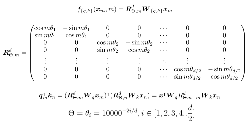
You need to look at RoPE’s formulas (see the cited section). RoPE does not simply rotate a token vector by a single angle; instead, the token vector is first split into a series of 2D components, and each 2D component rotates at a different speed. For token positions, low-dimensional components rotate fast and high-dimensional components rotate slowly, like the second, minute, and hour hands of a clock. A single component’s rotation is periodic, but the full token is unlikely to suffer a cycle collision.
-
Low-dimensional components rotate quickly, while high-dimensional components rotate slowly. This causes the low-dimensional components of the token vector to focus on local information in the sentence, while the high-dimensional components focus on the sentence’s global semantics. Embeddings themselves do not require different behaviors from low- and high-dimensional components, but a Transformer’s embeddings are learned together with the Transformer. This allows token vectors to differentiate in learning proximity within the sentence.
(The RoPE formula, image taken from the RoPE paper.)
Quote
- [4] 位置编码详解: https://medium.com/thedeephub/positional-encoding-explained-a-deep-dive-into-transformer-pe-65cfe8cfe10b
- [19] RoPE paper:https://arxiv.org/abs/2104.09864
Mixture of Experts (MoE)
The DeepSeek paper also explains in detail how production-grade Mixture-of-Experts (MoE) is implemented. MoE has become a standard for the next generation of large models, enabling much larger parameter counts and sparse activation. In MoE, the FFE layer of the Transformer block is replaced by an MoE layer:
-
Unlike a single dense FFE layer, MoE splits the FFE into many smaller FFE modules called “experts.” Experts can be activated simultaneously and are computed in parallel (Expert Parallelism).
-
For a given input token, only a subset of experts are activated. This is where the “sparsity” comes in: compared to the huge total parameter count, the cost of training and inference is greatly reduced.
-
Some experts are always activated; they are referred to as shared experts.
-
MoE introduces a router, which is the key component of MoE. The router must ensure load balancing, select affinity experts for tokens, and even take device and network overhead into account.
Each layer of DeepSeek-V3’s MoE has 256 experts; an input token will activate 8 experts plus shared experts, and each expert’s outputs are merged.
(DeepSeek MoE architecture, from the DeepSeek-V3 paper.)
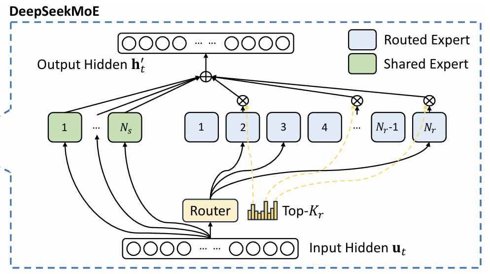
How does MoE perform routing? See the formula in the figure below:
-
u_t denotes the input token, and h_t’ denotes the output of the MoE.
-
Each expert has a centroid vector, denoted e_i. The similarity between the centroid vector and the input token represents the affinity between the input and the expert. The Top-K experts with the highest affinity are activated, called gates g_i,t.
-
The centroid vectors are trained together with the experts. The actual gating must also handle load imbalance, adding correction terms and penalties for load imbalance. See equations (16)–(20) in the DeepSeek-V3 paper.
-
From the above, routing can be expressed as matrix operations plus an activation function (Sigmoid). In other words, the routing module is also a (very small) neural network; the expert centroids are its trainable parameters, and the output can use Softmax to sample activated experts.
-
In the formula for h_t’, the experts’ outputs are added directly to obtain the result. FFN_i^(s) are shared experts and they are not gated. In addition, the input u_t is also added; this is a residual connection.
MoE is often challenging when it comes to balancing expert load. Expert collapse (a few experts receiving most of the tokens) and expert starvation (some experts being undertrained) are common problems in routing training. It can also be observed that MoE helps reduce the number of activations, reduce computation, and enable expert parallelism, but it does not directly reduce memory consumption because all experts still need to be loaded.
(The DeepSeek MoE formula, taken from the DeepSeek-V3 paper.)

Why apply MoE to the FFN layers instead of splitting the Attention layers? On one hand, FFN layers process tokens one by one, making them easier to split, whereas Attention operates on token pairs. On the other hand, FFN layers account for the majority of a Transformer’s parameters, far more than Attention.
(DeepSeek MoE 的参数数量 ,链接:https://mp.weixin.qq.com/s/WXrgxV3LgYYvRLPTVzLkjw )

Quote
- [20] Deepseek Technical Interpretation (3) - The Evolutionary Path of MoE: https://zhuanlan.zhihu.com/p/18565423596
- [21] DeepSeek-V3/R1推理效率分析: https://mp.weixin.qq.com/s/WXrgxV3LgYYvRLPTVzLkjw
Summary
End of text. Up to this point, we have introduced the fundamentals of Transformers, covering model architecture, neural network layers, Attention, and KV Cache, and we have also discussed the more advanced MLA and MoE. The DeepSeek paper provides a detailed account of large models from model design to infrastructure and is well worth reading. Polo Club’s visual Transformer offers interactive visualization, which is very convenient for learning.
Create an Issue or comment below
